On this Page:
- Input Value Panel
- Target Values and Formula
- Stock and Bank Account Values
- A short excurce in Prediction Theory
- Catalog Values
- Detail Input Panel
- Result Graph Panel
- Detail Value Table
Input Values
![]()
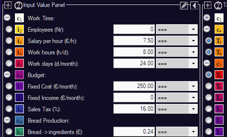
On the left side of the main window of Predicted Desire, you see the Input Value Panel, a dynamic list of all Input Parameters of your current Simulation Model.
An Input Value in Dynamic Applications consists of a Radio Button, Title, Unit, current Value, and estimated development Mode.
In brief, an Input Value is basically every item circle on a Balanced Scorecard that features only outgoing connections, i.e. arrows leading towards other items. Obviously, that item is an “influencer”, an Input Value (also called Input Parameter). In System Dynamics, it influences a Target Value, described by a formula where that input parameter occurs.
. ..

.. .
The standard application includes the Bakery Model, simulating a Startup producing a single product, called Bread. You’ll find here all Input Values of the Bakery model’s Balanced Scorecard, which describes the simulation’s logic between Input and Target Variables.
By clicking on its Radio Button, you can switch an Input Value or a Target Value on or off in the Result Graph Panel. Should the Radio Button be replaced by the Pencil Editor Symbol, you can still toggle Input and Target Values on and off by performing a Right Mouse Button Click.
In System Dynamics Applications, Input Values are referred to as Auxiliary variables.
. ..

.. .
The special thing about a System Dynamics application is that it allows you to change any Input Value over time. Like it is standard in Nature, but completely neglected or ignored in so many common, standard computer software applications. Next to the TextBox for entering a value, there is a value mode selector:
- stable (‘===’): stable over time (default setting).
- up | down: linear up or linear down, increase or decrease of the value over time.
- square | sqroot: will apply a square (x^2) or square root function over time.
- exponential will apply an exponential function, the strongest raise we know.
- saturated starts like an exponential function that then nears its limits to growth.
- bell-curved gives a local maximum, a hill, derived from the Gaussian Distribution.
- trending simulates an overshooting trend curve, a damped oscillation frequency.
- free steps allows you to manually set a custom value for each time step.
Here, you can enter a predicted development of a single parameter, like fine-tuning a screw of your company’s simulation model. About every company, every startup, every person is an expert into the things they do, regularly. They know them well. Who else could predict an input parameter’s development, if not you?
The basic achievement of Predicted Desire is that it allows you to focus on fine-tuning the single parameters, only. The calculation engine of will care for calculating all the influences that this value has on the various Target Values reached directly or indirectly from here.
If you are unsure about the meaning of an Input Value, move the mouse over its coloured [i] icon. An explanatory ToolTip will show up with basic information about the current value. Even if ToolTips are deactivated in the Options menu, you can always click on a coloured [i], [T] or [S] icon. This will force the ToolTip to display, manually.
All Input Values follow a standard pattern, here. For the application, an input value is basically a value with a title label (including the unit), and its development mode. It allows you to diversify any given value over time as part of the standard product. Predicted Desire doesn’t have to know its meaning; instead, it just applies all the formula that depend on this value, and calculates their results. A Balanced Scorecard with all its Formula and Input Parameters filled in is sufficient to describe the calculation as a whole, on a sheet of paper. A list of Input Values, and another list of Target Value declarations with Formula, is enough to describe the calulation, technically.
When entering an Input Value, or modifying its development mode, the value will be pre-selected for display in the Result Graphics Panel, as well as shown in the Detail Input Panel. We assume you are interested in investigating that value in more detail. In case you don’t want to see the value in the results panel, simply un-check its Radio Button on the left.
Also, you’ll see a question mark (trending?) in the mode selector. It will remind you that this mode is now in detail investigation. The (?) will go away as soon as you commit your selection using the green checkbox in the Detail Input Panel (accept), or choose some other variable to modify (cancel). This is to assure that you wouldn’t accidentally destroy your parametrization.
. ..
.. .
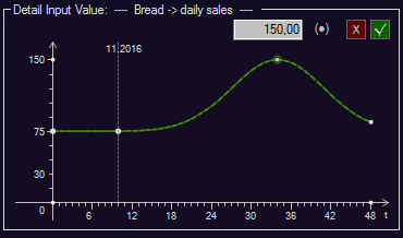
In the Detail Input Panel, you’ll see three number input fields at the top. The first one is the starting value, the value at the current Time Ruler position (e.g. t=0). The middle input field shows the curve’s reference point, the maximum or final value that the progression will reach. It’s very important to enter here a suitable, realistic value you want to achieve. Per default, PD suggests that you’ll be able to double the starting value within the given time period, a raise of 100%. For example, it may be realistic for a startup to ramp up production by 100% within 48 or even 24 months.
But why should it slow down again? – the bell-curved mode does make sense if you expect an intermediate rise of production. In most standard cases, choose from the linear up, squared, sqroot, exponential, or saturated rising modes:
. ..
.. .
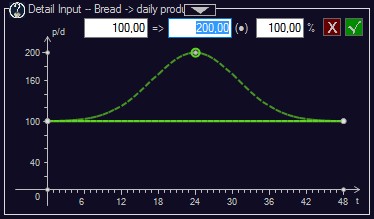
So here, we expect a rise in production from 75 products per day to 150 products per day within 48 months, a rise of 100%. You may now adjust the rise or fall in %, or by absolute numbers. Negative values are allowed in most cases, so you could also enter -50 percent to end up at half production, or -100 percent and your production will stop at zero units. As well, modify the starting or the reference value and the percentage will update, automatically.
It is very important to think about what seems realistic, here. If you ramp up production from 75 to 300 units, i.e. by factor 4 and raise of 300%, PD will tell you that production will cost you 4 times as much. If you then ramp up sales also by factor 4, PD will tell you that you’ll earn a lot more money within 4 years. In theory, this is an absolutely precise result, considering fixed cost influence and all! If you fail to ramp up your production by factor 4 though, it may happen that you end up in a completely different situation. In practice though, ask yourself the following questions:
- is it realistic to achieve this goal within the given time frame?
- are there any side effects? –
- check daily production time, you may need more workers!
- maybe you’ll need better material, or more energy: adjust those as well!
- remember that you may check all formula by tipping on the [T] icons.
- before turning your company around, check if all formula apply to your situation.
As you see, System Dynamics is not a crystal-ball approach. You get a perfect prediction if you know what you are doing. We assume you know your product, or it should be possible to talk to your engineers and find out about it. What PD does is that it relieves you from counting all these small effects together, that make up your company as a whole. You can concentrate on each singular parameter. Define a realistic future scenario by starting from today. What would be possible today if we got better machines, material, etc? – there you go. The only extra thing you need to consider is how long is it gonna take you to get there.
. ..
.. .
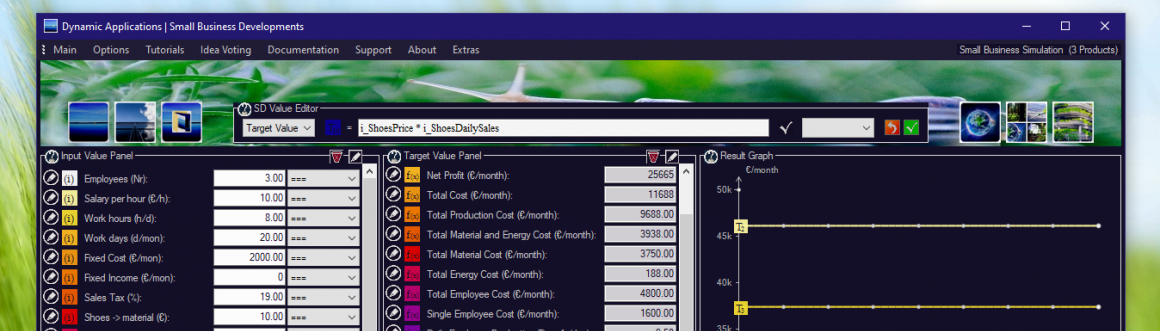
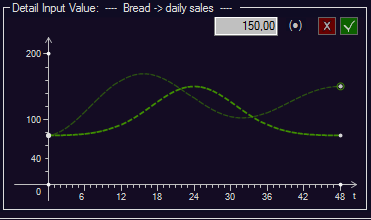
One important thing to know is that you can always move the Time Ruler forward. In the screenshot above, the user has started a progression (100 => 200) with 100% rise. Then, he or she moved the Time Ruler forward. This way, the Time Ruler has started progressing along the given curve, which may or may not be what you want.
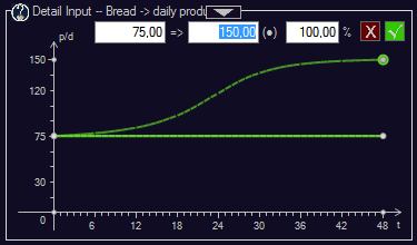
Alternatively, try to move the Time Ruler, first. This way, all values will stay stable at 100, as it uses to be in stable (===) mode. Move the Time Ruler to t=12. If you now switch the Mode selector, the Detail Input Panel will again open up, at t=12, but this time start from a constant 100 products/day for the first 12 months, then start climbing up to 200 products/day, reached after 36 months, and then continue climbing down the hill.
In free steps mode, when entering a value, the time ruler will move forward automatically. This allows you to enter one value after each other, by just hitting return after each value. Another way to achieve this is the Detail Value Table panel. Here, click into the field you want to start from, enter your value, hit return, and it’ll directly focus on the next value.
After having committed the Detail Input Panel by hitting the green checkmark, the current Input Value shown in the Input Value Panel will still show the starting value. But if you now move the central Time Ruler forward, it will start moving and always reflect the current value at that point in time.
This is because an Input Value can be different on each moment of time. All values that we observe in Nature would dynamically change all the time, even if the slightest. For ease of understanding, human has developed the typical time units we all know, from second to year, while time flows continuosly. Followed from that, there are rarely ever more than 100 steps on the time ruler, no matter what the simulation model is, as noone would build a simulation model with such a huge number of singular steps. Instead, you’d just redefine the time unit and use e.g. years instead of months.
If you want to see the progression of a single value, just open the Detail Value Table at the bottom of the screen. There you go – a long line of values, one for each moment in time, similar to an Excel Table.
In PD though, you could also look at your curve in the Results Graph Panel. The solver within PD is working so fast that we are showing live predictions. Your values should always be in Sync with each other, no matter what Panel you choose to look at.
In the Detail Input Panel and Result Graphics Panel, an Input Value will be painted using a dashed line (- – -).
Target Values and Formula
![]()
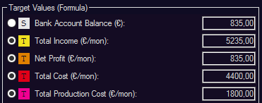
A Target Value in Dynamic Applications consists of a Radio Button, a Title, a Unit, a Formula, and a current Value. As explained above, basically every item on a Balanced Scorecard with in-going parameters, results in a Target Value in Predicted Desire.
There are two types of Target Values: simple Target Values (T), and Stock Values (S).
In System Dynamics literature, Target Values are often referred to as Flows. As we all know, if we look at nature and even technology over a large enough amount of time, everything will flow. Nevertheless, for ease of understanding, we call them Target Values.
As for Stock Values, these are collecting values much like a Stock is collecting bees, so we keep close to the System Dynamics definition, here. See below for more.
. ..
.. .
Target Values (T):
The Formula will show up if you move the mouse over the coloured icon. A formula in SD can contain any number of input values, or other (sub-) formula. As you can see, Predicted Desire contains an algorithmic engine that will solve each of the formula from the list of target value, automatically. By then, it will know about the complete formula to calculate the current value from. This is possible if there is not an inner circle of formula depending on each other. That would only be possible if there was a time delay within the circle’s calcultion (we plan to support that, later). Within a Balanced Scorecard, there’s always a hierarchy within the formula system, resulting in a clear path of calculation of a value.
As a Target Value is always calculated, it is not possible to enter a value, manually.
To influence a Target Value, look up its formula (as shown in tooltip) and find the correct Input Value that you really want to change. In the tooltip, you’ll also see the formula resolved to a lengthy expression. This is only to give you an idea about the real calculation formula. Very long lines will be abbreviated by ‘…’, and you don’t want to read them.
Our Formula Solver will automatically resove and calculate all values for you.
For a detailed description of mathematical expressions supported in a Formula, please refer to the Desire Language Specification guide.
.. .
Whenever you move the Time Ruler, the solver will calculate through all its formula, and show you their resulting, current Target Value at that moment in time.
In the Detail Input Panel and Result Graphics Panel, a Target Value will be painted using a solid line with white dots (●-●-●-●).
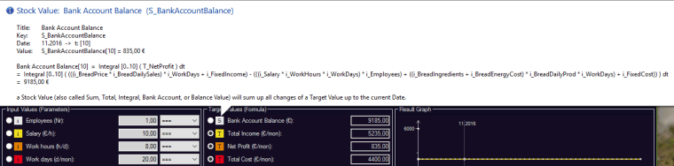
Stock Values (S):
![]()
While simple targets just caluculate the current value in time, a Stock Value accumulates values over time. So a Stock Value is defined by referencing a Target Value to sum up, or two targets: one Target Value to add upon, another Target Value that deducts from the stock.
You can picture it as a Stock of Bees, accumulating all the bees flying in, minus the bees flying out. As well, as a Bank Account, accumulating all arriving income in a single month, minus all the cost deductions of a single month.
. ..
.. .
In the picture shown, the Stock Value called Bank Account Balance will sum up the Net Profit Target Value over time. At the starting point (t=0), the value would be equal to the first month’s net income. In the next step (t=1), the value the first and second month’s input, altogether. After 48 months, it would be total to a 4 year’s income.
In the Detail Input Panel and Result Graphics Panel, a Stock Value will also be painted using a solid line with white dots (●-●-●-●), just as any other Target Value. Although it has a different way of construction, it’s really used in the same way:
both represent results of calculation.
See the following video that explains easily the difference between Stocks (Bathtub), In-Flow (Input (or Target) Variables) and Out-Flow (Target Variables) of a calculation model over time.
. ..
A short excurse in Prediction Theory
![]()
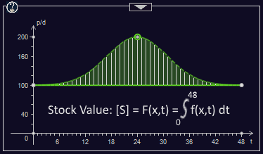
Mathematically spoken, a Stock Value accumulates all the different interval values of a function over time. We call that an Integral Function over the target value’s formula. An equation including a Stock Value is therefore called a Differential Equation.
The automatic equation solver of Predicted Desire is able to resolve a set of coupled, linear, or non-linear Differential Equations. This is of course a heuristic (simplifying) approach. The equations are not solved mathematically, where one would be searching for simpler equations converting to the same result. Instead, the Solver just inserts the resulting set of Input Values at the correct moment in time, and deliveres results near to the perfect solution. As in Math, the result would be the more precise, the more time steps we choose to simulate. This works exactly like the integration of a function over time, calculating the function’s area:
. ..
.. .
If you simulate the developments of a company, you could define all Input Values in hourly income. Within 48 months, a huge amount of hours would accumulate. However, no real person would be able to guess upon a company development over 48 months on a daily, hourly, or even smaller basis. So we choose months and get a prediction in good approximation. As we choose to simulate in a monthly interval, we’d also interprete all input and target values on a monthly basis. So, the accumulation of monthly income, accumulating all days and hours where money came in, would be done by the user when setting up their Input Values, naturally.
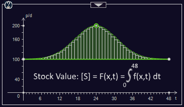
This is also why we chose for rectangular integration in the standard product: this way, everyone can verify a Stock Value by performing a sum-up of the underlying Target Values with a pocket calculator.
. ..
.. .
This way, we achive Perfect Prediction without having to look at infinitely small timed intervals. We define a perfect prediction as giving the exact results over time as long as all the single value developments were approximated, correctly.
In theory, we could also use a more sophisticated method of integration, like Euler’s integration. In the simplest case, this would use diagonal connections at the top of each rectangle, which would approximate the real function more closely. A variant that is really easy to calculate, with the trade-off of a more difficult verification for our users. Overall, the difference of both integrals should come down to a very few percent, and considering that we have a lot of unknown dependencies when thinking about future developments, we thought that rectangular integration is just perfect for most real-life cases.
As almost all the formula in a typical System Dynamics application do consist of simple addition and multiplication of monetary values, we typically get fairly good results if we are able to approximate their development, nearby.
Even if we use an exponential value development with a strongly accelerating value, as long as the dependent Formula do consist of linear addition and multiplication (typical), we get very good predictions if we just manage to estimate every single value’s increase.
Remember that we use Stock Values for any kind of accumulating function, like real-life bank accounts (money), stocks, piles, and stacks (material), or total balance of a situation.
Typically, in every simulation model you’d expect at least one Stock Value. It’ll show you the development of your most interesting Target Value, like your Net Profit development 0ver time, the total amortization of your PV System, etc.
System Dynamics is a Sustainability approach. It’s all about keeping your World in Balance.
Catalog Values

Starting from v7.42, Dynamic Applications introduces Catalog Values.
These are additional values that can be inserted via the small, top-left [+] icon in the SD Value Panel’s top icon line. Catalog Values are just carrying a catalog title, so they don’t feature a unit, a concrete value, or a mode selector.
Catalog Values are used to group Input and Target Values of similar Topic. Through a simple, intuitive [+] and [-] folding of all values below – up to the next catalog group – they provide for a well-sorted view as well suitable for more complex Simulation Models featuring long rows of Input and Target Values. When Catalog Values are active, their radio button icon is draw a bit leftwards, while all other radio button activators are moved a bit rightwards, automatically.
.. .
. ..
This handsome design underlines the impression of sortability of Input and Target Values by catalog.
Once inserted, Catalog Values can be moved up and down to their desired location, easily. Once placed at the right location, they can be accepted by hitting the green checkmark icon. Now, a new Catalog Value can be inserted by using the top-left (global) [+] icon.
Should a Catalog Value ever have been inserted that you want to remove, you can use the traditional remove method by activating the global Editor Pencil from the top right icons, then activating the global delete Icon (Trashcan) that will give each Value a small trashcan.
Catalog Values as well get a small Trashcan and so can easily be removed now, as well as they can be re-sorted or re-named by going back to standard Pencil Editor mode.
Detail Input Panel
![]()
The Detail Input Panel allows you to to fine-tune (predict) each single Input Value. It will be automatically activated as soon as you activate an Input Value by selecting its RadioButton, entering its Value TextBox, or modifying its development Mode ComboBox.
. ..

.. .
The Detail Input Panel will apply the current Mode selection to the value.
. ..
.. .
As you can see, the current value (75.00) from the Input Value Panel will be used as a starting point. For the remaining simulation time, the selected mode’s development curve will be applied.
Please note that you always have to accept any value’s modification by clicking the green checkmark icon on the Detail Input Panel. Otherwise, it will be temporary shown on the Detail Input Panel. The new curve will be transferred to the original Input Value only if you confirm the mode change by clicking the green checkmark icon.
This will allow you to toggle through a couple of modes and select the right development curve, without destroying any current values. If you change your mind, there’s always the red cross cancel icon. It will perform a simple undo to the last confirmed value.
The red cross cancel icon will reset the curve to the last confirmed state, as well as notify the original Input Value, which will also reset its mode selector.
. ..
.. .
The Default Scaling (2x) of your Input Value will be automatically adjusted so that the maximum value approximated by the chosen curve will be twice the current value.
In the example, the current value is 75 daily sales, so the maximum value will be 150 daily sales. This is true for all the functions in the list, so that we can switch development modes and still get comparable results by default.
The (o) circle marker will identify the reference value of the associated curve and allow you to enter a different, more appropriate reference value to reach, in the TextBox. The scaling of the curve will then be automatically re-calculated, the curve will be adjusted to reach your chosen value, and you may see the scaling of the y axis being changed, accordingly.
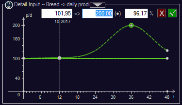
The trending mode (trend curve) is an exception, as we got an overshoot here: the maximum is even higher as the reference point. It is typical for a real Trend Curve to result in a first hype, then fall down to the valley of depression, and finally reach the productive target we’re interested in. System Dynamics is a sustainability approach, and we’re always interested in long-term developments.
The other exception here is the down mode that will lead to half (0.5x) the current value.
In free steps mode, an automatic maximum doesn’t make sense as this mode is for entering manual, freely chosen steps, yourself. Here, you’ll see the Current Value in the selector box, and you can enter every next value, manually. As soon as you enter a value, the central Time Ruler will move forward to the next step. You can accept the same value by just hitting enter, or type in a new value for that step.
Result Graph Panel
![]()
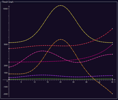
The Result Graph Panel will show the development of all Input and Target Values within the simulation time period.
. ..
.. .
The x Axis of the Result Graph shows the development of Input and Target Values over time.
The y Axis of the Result Graph will show the function values, i.e. the Target Values as calculated by their associated detail Formula. Each value will be represented at its point in time on chart; however, a comparison of values does only really make sense if you choose values bearing the same Value Unit. Still, it’s possible to display all kinds of values, as it may be a useful visual feedback when adjusting the single Input Values.
At the moment, there is no real distinction between the values. As a hint though, each value has got its own formula. Target Values will show a line of white dots, Input Values will show a dashed line.
To find out about a specific curve, simply toggle (deactivate) any Input or Target Value with a matching colour. To find out about specific detail values, check the Detail Value Table section, below. It will automatically show the last activated value, also for Target Values.
A display curve in will be shown for every value that has got an activated Radio Button.
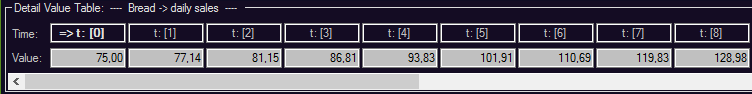
Detail Value Table
![]()
The Detail Value Table displays the most recently activated Input or Target Value’s development over time in detail.
. ..
.. .
The current Time will be highlighted with an arrow ( => t: [0] ), the value displayed will be shown in the title bar (‘Bread -> daily sales’).
The Value line will show a single value’s development in all iterations over time.
In case of selecting an Input Value, you can click into any field to adjust that value, manually. The central Time Ruler will move forward automatically, so you can directly continue and adjust the next value.
In case of selecting a Target (or Stock) Value, all values will be presented read-only.
. ..

.. .
In the example shown, you can see how the Bank Account Balance – a Stock Value – is accumulating the net profit value of 835.00 € over time.
Internally, all Input and Target Values are calculated in double precision. The values are rounded to two-digit display for financial application (currency). Large values (10000+) are automatically rounded to whole numbers, very large values use scientific notation (1.234e6). Small numbers are shown in detail (0.0015), very small numbers also use scientific notation (1.5e-7). This applies to all panels and result graphs of the application.
Navigation
Page 1 -> Top: Main User Interface – Model Selector – Time Ruler – User Voting
Page 2 -> Top: Input Values – Target Values – Formula – Result Graphics – Detail Values
Dynamic Applications.
![]()
Dynamic Applications is a small business consultancy focused on customers, product cost, efficiency, sales, and net profit. We support Startups in developing 21st century Business Models. We’re driven by thousands of independent voters. Altogether, we create Small Business Developments, an evolving platform of free and simple business plan calculators for everyone.
We vote in online democracy, we deliver for free. we work for you, and we call them Dynamic Applications.
at Dynamic Applications, we work to empower people.
we are Sharing Economy. Follow us to gain.
Thank you for choosing to visit Dynamic Applications, today. Comment section is open.
