PD Inline Formula Editor Documentation.

PD Inline Formula Editor Documentation.

So here we are, in April 2020, explaining our brand-new Inline Formula Editors in detail.

In the beginning, Dynamic Applications were basically empty. There was nothing but three large, dark, and empty fields. Input Value Panel, Target Value Panel, Result Graph Panel.

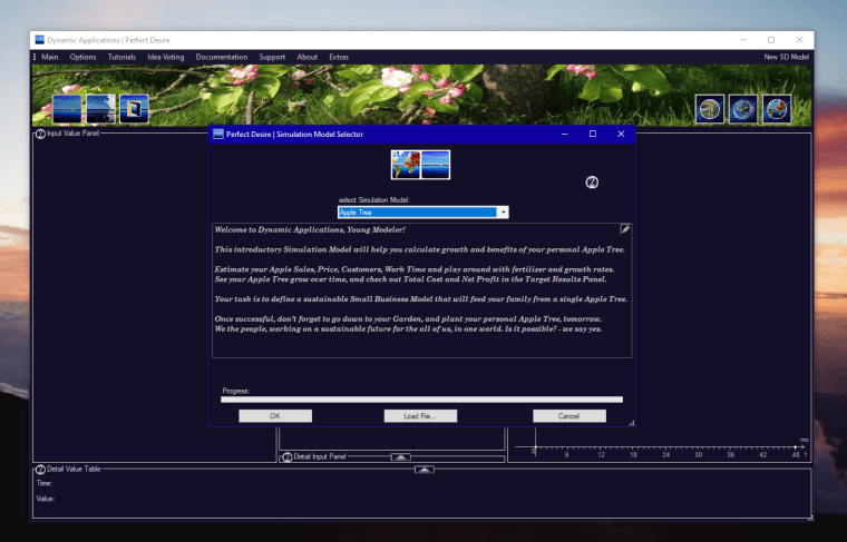
The program starts up with the Simulation Model Selector, showing all Simulations available in the User’s Document Home Folder, called XMILE. Here, your own Simulations can be saved. Below the line, all built-in Simulation Models are shown, as they come with every Dynamic Application. These are loaded on Startup, and thus create the list of Simulations.

Dynamic Applications are based on a Formula Language that we’ve called Desire, because it’s beautiful in its simplicity. It basically consists of common Mathematical Expressions, like [+][-][*][ / ], x^y, sin( x ), cos( x ), min( x, y ), max( x, y ), and ifzero( expr, then, else ).

In Desire, we can create any Number of Input Variables. Then, we can create Target Values that will be automatically evaluated and calculated. A Target Value may contain any number of expressions, may it be numbers, functions, Input and Target Values. 

In Desire, so an Input Value represents a Variable and a Target Value represents a function.

Then, as with every popular programming language, there’s cases to decide (if-then-else), and also there are ‘for( i=0; i < length; i++)’ loops. In Desire, instead of making complex formula with for loops, we simply create Stock Values.

See below for more.

---

---

Starting up a Simulation.

In Freeware Products, the first 12 Input and Target Values will be editable, so that you can try out everything in all cases. 

You can enter our Universal Promo Code to activate all Formulas. It’s hidden on various pages within our Website, and it’s shown in one Tweet of the Dynamic Idea and Roadmap Voting (.. @dynamic_idea  t  @dynamic_qs .. ) on Twitter.

All Windows 10 Store Apps and our 2 professional solutions, Small Business Developments and Perfect Desire, bring the full-featured Formula System. 

The professional version will officially support to create, modify, and remove Input, Target and Stock Values, and to load, save and run calculation models in x / y / t with up to 100 Input Values and 100 Target Formulas. That’s formally guaranteed by dna license.

Should something not work as expected here, you can report that as a bug, and it’s gonna be fixed free of charge (as soon as possible for users of the professional versions).

Now, in loading the selected Simulation, Dynamic Applications will read in the Simulation Model File, which contains basically a list of all Input and Target Formula Specifications.

For each Input Value and for each Target Formula, as well as for accumulating Stock Values (treated much like Targets here), a new UI element will be created, automatically:

Radio button, [i][T][S] Icon Symbol, Title, Unit, Value, and Mode Selector for Input Values.

Finally, the whole equation system, as described within the Simulation Model File, will be evaluated and resolved. That works much like you may have learned in School, when you’ve got a set of three unknown variables, in three equations, e.g.:

• a = 4 * b + c
• b = 2 * c
• c = 15

you can resolve this Equation System as follows:

• c = 15.
• b = 2 * c = 30.
• a = 4 * b + c = 135.

That’s pretty much what our Universal Equation Solver Engine does, automatically, when loading Dynamic Applications. Input Values are always known numbers, so they are inserted into Target Formulas. So Target Formulas become solvable. Finally, as soon as all Target Values are known, the Simulation Model Selector disappears, and your Dynamic Application of choice is up and running.

Now since the whole Formula System is being interpreted on-the-fly, we can also do live changes.

For this to activate, you have to click on the small [ / ] Pencil icons on Top of the Input and Target Value Panels. This will replace all Radio Buttons with Pencils.

Congratulations! You’re in Editing Mode, now.

..

---

Editing SD Values: Title, Unit, and default Value.

To Edit an Input or Target Value’s Title, Unit, default numeric value, or its Math Formula, first we have to activate all Editors by clicking the square [ / ] Pencil icon in the top-right corner of each SD Value Panel.

By clicking on one of the Pencils, the SD Value, as selected, will highlight it’s Title Editor field. So you can directly rename the item selected.

The (o) Radio Button Selection would normally activate an item, so to display its results in the Result Graph, as well as show all its values (t=0..48) in the bottom Detail Value Table.

In Pencil Mode, (de)activate Input and Target Values with the Right Mouse Button, instead.

In Professional Products (available for the Top 12 Elements in our Freeware), you’ll activate our Inline Formula Editor, which automatically replaces the central Time Ruler. 

We need a way to refer to any SD Value in our Math Formulas. In Dynamic Applications, such a Value’s Formula keyword will be derived directly from the item’s Title.

All SD Values will be prefixed i_InputValue, T_TargetValue, and S_StockValue, respectively.

• Input Value:    Employees => i_Employees
• Input Value:    My Employees => i_MyEmployees
• Target Value:    Net Profit => T_NetProfit. 
• Stock Value:    Bank Account Balance => S_BankAccountBalance.

Now your formula expression can be read easily, and keywords are defined, precisely. See below for more.

..

Creating New Input Values, New Target Values, or New Stock Values.

Whenever activate all Pencil Editors by selecting the Global Pencil Editor on the Panel’s Top, a New Input Value / New Target Value will appear at the bottom of each SD Value Panel. This way, you can easily add new Values to your calculation.

To activate such New Input Value / New Target Value, simply edit it’s Title. Otherwise they’ll disappear again when deactivating Editor Mode, because they haven’t even got a specific Title. 

Whenever you’ll accept a new SD Value by hitting its green OK checkmark, another New Input Value or New Target Value will appear, below. This way you can easily expand your Input and Target Formula System, step by step. In the Freeware products, we support to create, load and save Simulation Models with 42 Input and Target Values, altogether. In Professional Simulation Model Development (acquire Small Business Developments or one of our Windows 10 Store Apps), we support Simulation Models with up to 100 Input Values and 100 Target or Stock Values, respectively, which should be more than enough.

New Stock Values can be constructed from a New Target Value. 

To create a New Stock Value, activate its Pencil Editor, then change its Type to Stock Value in the Inline Formula Editor’s leftmost Value Type Selector. 

..

How to Remove an Input or Target Value.

Finally, with every Formula System in daily life, there’s also a need for removal. When activating the Pencils, a small, dark-red Recycle Bin symbol will appear next to it, on Top. Now if you click on that Top Recycle Bin, all Editor Pencils will show Recycle Bins. Now select your Recycle Bin of choice, and so destroy its value. 

If you delete an SD Value in use within our Target Formulas, you’ll be warned, beforehand. If you destroy an important value, nevertheless, all Targets wih invalid Formula will instantly show an Error Symbol [!/].

Click on the Target Value’s [T] Symbol Icon and a descriptive Formula Error Message will be shown in the Target’s ToolTip, automatically. 

Persistance and Resilience of Formula Systems in Dynamic Applications.

All Input and Target Values that are still functional and not affected by an Error Symbol will work, flawlessly. So you can always see where there is work to do. 

Now you can correct all your remaining Formulas, as desired, and as soon as the final formula is corrected, all [!/] Error Symbols will instantly be gone, again.

---

---

Specifying Units. Unit Conversions.

Next to its Title, each item also has a Unit description field.

So here you can enter a financial or physical Unit like Euro, kg, m, day, year, s, Euro / Month, or even a combined unit like m / s², km / h.

In Dynamic Applications, Units are only used for descriptive purposes. So they appear within ToolTips, as well as on the vertical axis of the Result Graph when selecting an element. But whatever you specify there, it will have no influence towards the calculation, by default. So the calculation results will not change if you change hour (h) by second (s). You can write hour, hours, h or second, sec, s as you prefer.

In theory, it would of course be possibly to apply automatic number conversions from hour to second, but then, think about converting days into months, it already would become difficult. An easy approach here would of course be to assume 30 days per month, average. However, in Dynamic Applications, for ease of operation and understandability, there is no automatic conversion. Such conversions will have the effect that every Unit must match exactly towards the internal conversion system, or there will be calculation errors. So that would require extra attention.

Instead, when using Dynamic Applications, we specify all Unit Calculations within the Formula, itself. That’s most easy and as good. So if you have one Formula using Gram (g), and one other formula using Kilogram (kg), there should be a  * 1000  conversion,  somewhere. If you have seconds and hours, there should be a 60 * 60, a conversion factor of 3600 within your formulas, where necessary. A separate Unit calculation system would have that same calculations, only separated. So here we have everything in one place.

In developing Dynamic Applications, we prefer understandability, ease of operation, and less complexity, reflecting Transparency and Participation, our project’s cultural guideline.

So we can talk of ‘Working hours per day’, and specify these in hours (Unit: h). Technically, if working with Unit conversions, the label would have to be called ‘Working’, and the Unit would have to be ‘h/day’, or the calculation system couldn’t resolve the Units, properly. So that’s why we keep it simple and you have one formula, and there’s no hidden calculations in the background.

To round up, we have the possibility to add any Unit description, but that will not have any effect on your calculation.

---

Changing Default Values.

As well as editing Titles and Units, you can also change the default Input Value. So if you change the number shown, then save the Simulation Model, it will load and run again with your preferred default value. 

Since Target Values are calculated, automatically (derived from Input Values and Formula), it will not be possible to change a Target Value, by number. Instead, you’ll have to change it’s calculating formula, accordingly.

While there have been frequent questions whether it would not be possible to allow for direct manipulation of Target Values, this will not be supported. Yes. In theory, it would be possible to enter a different number, and see it’s outcome, on the spot. But that could easily bring the whole formula system out-of-order. First of all, the value shown is just one value in a 48 – to – 100 value combination, depending on the number of Time steps. If you want to change singular Input Values for a specific time, you can do that in the bottom Detail Value Table, which works much like a line of Input Cells in Excel. Just enter your numbers, one by one.

However, changing values for Targets would also mean that the incoming formula system must be cut away. Still, the Input Values in question could have effects on other Formula. This may or may not be obvious in the given case. Generally spoken, the effects of manipulating a specific Target Value’s display value would be uncertain, and almost undiscoverable (if not following all the ToolTips and thereby understanding all dependencies of the whole Formula System). So we better forget about it.

In Dynamic Applications, for clarity and understandability:

• Input Values are Parameters and can be edited with a Pencil’s click, then accepted.
• Target Values are calculated formulas and they so they can not be edited.

..

---

Moving Input and Target Values, up and down.

   

The final User Interface field is now replaced by these 4 symbols:  up, down, undo, ok.

These will operate much as expected: 

• move down will move an item down the list. It’s index nr will increase by 1.
• move up will move an item up the list. It’s index nr will decrease by 1.
• undo icon will undo your latest changes, so the icon’s name, unit and value will be restored.
• checkmark will accept all your changes. Undo will then restore the accepted value.

If you move an Input Value beyond the Top or Bottom of the list, it will toggle around, and appear on the other (Bottom / Top) side of the list, automatically. 

The index numbers of  your Input and Target Value Panel are always counting from Top, starting from 1..2..3..4..5.. … towards ..n-1..n, for n elements. So the topmost Input Value will always be white, and show [ i₁ ].  The next one will always show [ i₂ ]. So when moving an item up or down, it will exchange its place, as well as its index number, with that neighbor. So that virtually only the item Title, Unit and Value are changed, but colour and index will always stay in place, as they are always sorted in order of appearance.

For convenience, you may also click the right mouse button and move an item up or down by +/- 10 positions, at once. As well, its index number will increase or decrease by 10 in this case.

Following each checkmark acceptance, there will be a Target Formula Evaluation for all Targets. So if you have introduced any error, all defect locations will now be shown, with their values showing -/-.

Nevertheless, the remaining Formula System shall work as specified, undisturbed.

That’s what we call Persistence.

..

---

Editing and Specifying Formulas in Dynamic Applications.

To be able to specify Formulas, we need a way to display Input and Target Value Titles.

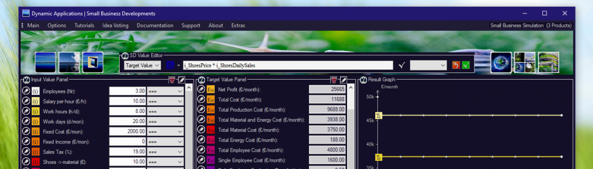
For ease of operation, simply click on an Input or Target Value’s Icon Symbol ([ i ], [T], [S]), and the associated Target Formula descriptor will appear in the Formula Editor.

For this purpose, and for ease of operation, a matching Formula descriptor will be created directly from the item’s Title. 

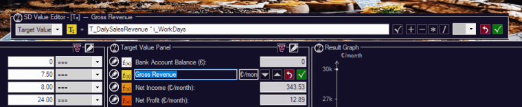
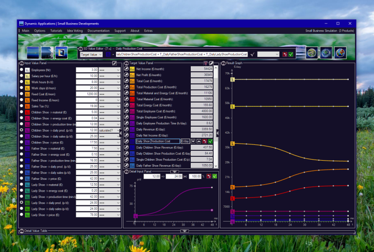
In the picture below, by clicking on ‘[T] Total Cost’, the Target descriptor T_TotalCost appears.

Now if you change a Target Value title from ‘Gross Revenue’ to ‘Gross Margin’, it will change automatically its formula descriptor from T_GrossRevenue to T_GrossMargin, throughout the whole formula system. Where ever T_GrossRevenue was mentioned in a formula, it is automatically replaced.

While creating the formula descriptor, blank space and non-characters like ‘,’ and ‘->’ will be ignored. For ease of interpretation, each single word is now drawn together, capitalized:

• Bread, Production Time  =>  i_BreadProductionTime
• Bread -> Daily Sales  =>  i_BreadDailySales
• Sales per hour  =>  i_SalesPerHour
• Net Profit   =>  T_NetProfit
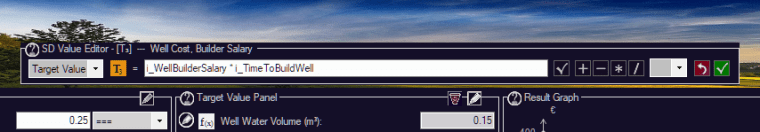
• Time to build Well  =>  i_TimeToBuildWell

Each Formula descriptor will be prefixed by either of  i_, T_ or S_, representing Input, Target and Stock Values, respectively. So there’s a clear identification of elements in a Formula. 

The very nice side-effect of this is that you never have to care for the Value’s Formula descriptor, explicitly. It will always be automatic. A small drawback that comes with this simplification will be that when creating Multi-Language Simulation Models, each Language will have its own Formula Descriptors (readable in the local language). 

We recommend to create different Simulation Model Files for each language in this case. Still, it is very well possible to create a Simulation Model in one language (e.g. English), then save that reference Model to disk. Then, load it again, activate all Pencils, translate all items to German, French, Spanish or Russian Language, and save that resulting model, named in its local language. This way, the formula system will adapt automatically to each language, so you can simply translate the User Interface Titles, save it under a new name, and that’s already all. Now you have one English and one German Simulation Model.

Apart from that specific consideration, a great benefit that comes from automated Formula descriptors is that you can highlight each Formula descriptor by a single (or double) mouse click:

Now that you’ve highlighted an Input or Target Value, for easiness of operation, you can simply click on an element’s ToolTip symbol to add it right in place of that highlighted symbol, at the Cursor position.

In using the integrated [+][ – ][ * ][ / ] symbols, as well, this way you can set up any simple formula, without using the keyboard, at all. Of course, we also support brackets ( ), ^ for power, or any number you want to add or multiply. As the space for editing your formula is quite limited, these you’ll have to type in using your keyboard, though.

Please note that both editing systems (Title, Unit and Value Editors, vs. Formula Editor) are mostly independent of each other. Accepting a Formula will automatically influence a Target’s ToolTip, and changing a Title will also influence its automated Formula descriptor.

For this reason, the whole Target Formula system will be evaluated after each click on a checkmark. For easiness of operation, the Target Formula will as well be evaluated when hitting Return. So here you can already see whether you have got a valid formula, without leaving the keyboard.

The Inline Formula Editor can as well be used for editing Input Values. Here, there is no formula, so you can edit directly its value, as well as its comment. To edit an Input or Target Value’s comment, please choose ‘Comment’ in the Editing Mode selector on the left.

..

---

The Theory of Stock Values.

 

In System Dynamics, Stock Values are automated counters. There are many applications for these. The most easy explanation for a Stock Value will be a Stock of Bees. Whenever a new bee arrives, the Stock Value accumulates by 1, because there is now 1 more bee within the Stock. When 2 bees appear and fly into the Stock, it’s value will increase by 2. When 3 bees departure for collecting honey, the Stock Value will decrease by 3. So the value of a Stock is not 3, instead its value will always depend on its previous value, the value at [t-1].

If there were 100 bees in the Stock, and 3 bees would departure, we’ll now have 97 bees in stock.

Since we will have situations where we want to describe a start value, start position, or starting velocity, to name a few examples, there is another Selection Mode below ‘Stock Value’, called ‘(S) Start Value’. Here you can specify an initial value of Bees for your Stock at the starting point of your simulation, [t=0]. So you can start your simulation with 100 bees.

As well, you can use Stock Values to describe any accumulating value.

Like a Target Value, a Stock Value is specified by evaluating its own formula from t=0 to t. With the central Time Ruler, you can view every single result of the underlying ‘for’-loop, looking at the sum of all earlier Formula Values, calculated in Time interval from [0..t-1]. Since we’re calculating over time, this is already, mathematically seen, solving an Integral of Target Values over time. But as i said – we can also view this as a Stock of Bees.

Every Stock has got a Start Value: S₀.
Here we define the initial number of Bees, by number, or by single Input or Target keyword.

Then, from t=0 to t=1, any number of Bees could arrive or leave the Stock. So that changes our number of bees in Stock, over time. So a Stock Value is nothing less than a simple counter.

• S_FirstStockValue = S₀ + Sum( 1 ).
• S_FirstStockValue = 0, 1, 2, 3, 4, 5, 6, 7, 8, 9, 10, …  (with S₀ = 0).

Much like it works with Monthly Profits stored on your personal Bank Account, keep in mind that a bee has to arrive at Stock first, before it counts.

Therefore, at a given Time t, a Stock Value will carry its Start Value, plus the sum of all Bees having arrived before, minus the sum of all Bees having departed over time. 

Let’s take a look at a simple example. A number of Arriving Bees (described by some other formula) is arriving and occupying an empty Stock of Bees.

• S_StockOfBees = T_ArrivingBees
• Please note that in the first month, the number of bees in Stock would here be 0.
• with T_ArrivingBees = 0, 0, 0, 0, 5, 10, 20, 25, 100, 25, 20, 10, 5, 10, 100, 75.
• => S_StockOfBees = 0, 0, 0, 0, 0, 5, 15, 30, 50, 75, 175, 200, 220, 235, 245, 250, 260, 270. 
• The final number of T_ArrivingBees (the final 75), can and will not yet be respected.

In Reality, there’s also History. Let us consider an initial Stock (Start Value) of 100 Bees.
Then, let’s assume that at every Time t, one new bee is born right within Stock.
Here, we define an original Stock of 100 Values.
Then, with every Step in Time, we have to add T_ArrivingBees[t-1], plus 1 new bee.

• S_StockOfBees = S(t) = Sum( T_AttackingBees + 1), with S₀ = 100 Bees.
• T_AttackingBees = 0, 0, 0, 0, 5, 10, 20, 25, 100, 25, 20, 10, 5, 0, 10, 100, 75.
• S_StockOfBees = 100, 101, 102, 103, 104, 106, 117, 138, 164, 265, 291, 302, 308, 309, 320, 421.

So now you know everything about Desire, our beautiful, most simple programming language. It’s very simple, in that it can only calculate formulas in plain Math.

But for that purpose, it’s a quite powerful language, already.

• Variables:    supports up to 100 Input Variables.
• Functions:    supports up to 100 Target Variables with Formula.
• Conditions:    supports decisions: ifzero( expr, then, else ) and ifpositive( expr, then, else ).
• Formula Solver:    a Target Formula may refer any number of Input Variables and other Formula.
• Recursion:    a Target Formula may access all TargetValues[0..n], including itself[T-1].

By the way, not to forget:

in allowing us to estimate the development of any single SD Input Value over time, 

well, well, we don’t know everything. You may be 10% wrong here, 10% below there. 

But all in all, Dynamic Applications will calculate the Statistical Median Expected Value of all your assumptions. At Scientific Institutes, that’s the best and most precise known method of planning a business. 

However, this is a do-it-yourself approach.
We don’t believe in Politicians, Scientists, or People on TV.
Think self, here we say. At Dynamic Applications, we are collecting facts.
Dynamic Applications have been created to support any level of User Experience.
Good for our Products, good for planning your Startup, good for all your Customers.
So from all we can tell, in predicting results over time, keep looking out for reliable facts.
Describe any behavior of Dynamic Systems in time, may it be Business, Science or Nature.

Starting up your own Business, one day you’ll understand why understanding, addressing of your customer’s needs is a Win-Win-Win Situation.

Keep looking out for creating such Win-Win Scenarios, yourself. Take any given Simulation Model, rename and create new Input Values, Target Formula, or even be able to calculate Differential Equations of higher degree with Stock Values, in fine resolution. In creating your first own business, keep in mind that 90% of all Startups will close down or even go bankrupt within the first 4 years. Here, we target the remaining 10%. True winners.

So Take a look on how to lower your Costs, and calculate a fine price to deliver, from day one.

Good luck on your Endeavours, where ever from you may be visiting us, today.

---

---

---

---

Creating and Editing Stock Values in the Dynamic Applications User Interface.

Let us define a Bank Account Balance that should accumulate your Net Profit. 

First of all, delete the Bank Account Balance, should it be there. As nothing usually depends on it, that should be possible without causing any problems in the Target Formula system.

Or we could simply start from an Empty New Model.

Now, let’s hit the Pencil.

We take the free ‘New Target Value’ at the bottom, and name it ‘Bank Account Balance’. By moving it down the line once more, it will automatically toggle to the Top.

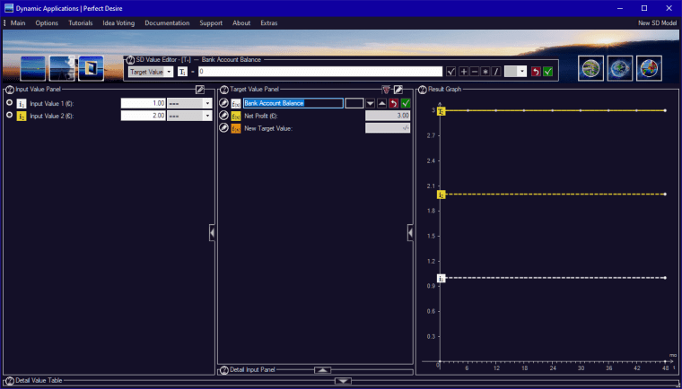
You can rename the other Target Value as ‘Net Profit’ by clicking on its Pencil, then accepting by hitting the green checkmark, before or afterwards.

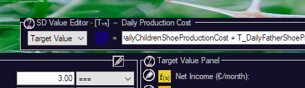
Now you create your Stock Value simply by changing the item’s Operation Mode in the Mode Selector on the Inline Formula Editor, top left. In the screenshot, it still shows ‘Target Value’. Please click on it, and select ‘Stock Value’.

Now, what do we want to accumulate? – Net Profit.

With one additional click on the yellow ToolTip symbol before ‘Net Profit’, you’ll have T_NetProfit inserted in the Formula Editor. 

That’s it, already! – your Stock Value will now accumulate Net Profit.

Now if you say, but you have 2500 Euro on your bank account, in the beginning, good for you. Select ‘Start Value’ and set that amount of 2500 to define the initial value, then accept.

Your Bank Account Balance should now represent in a diagonally upwards pointing line:

2500, 2503, 2506, 2509, 2512, 2515, 2518, 2521, 2524, …

As that is certainly not an attractive Profit, you can now change the Profit per Month.

In the standard New Empty Model, the first Target is calculated to be the sum of Input Value 1 and 2. So now you can enter any value for an Input, and check out the results, accumulating over time. So if you add 1000 and 2000, you’ll have earned 3000 Euros per Month, and your Bank Account Balance should go 2500, 5500, 8500, 11500, 14500, 17500, and so on. Much better. 

In traditional System Dynamics, a Stock Value is assumed to have an Inflow and an Outflow. So that’s best explained by a Water Reservoir, and it works much the same.

The Inflow is always added up, and the Outflow must be substracted. 

To simulate such a Stock Value, you simply specify this using ‘T_Income – T_Cost’, for example. 

In Dynamic Applications, for easiness of operation, we can as well specify about any other formula. Changing its Target Mode to become a Stock Value will just care for automatically adding up all its values over time, much like a Bank Account is collecting (adding up) and the money you pay in per month, and substracting any withdrawals.

You are welcome to try out, then create any Formula System that you may desire.

..

---

Specifying Math Formula in Desire.

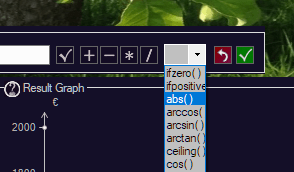
As of today, the following functions are available within the Input Formula Editor.

• [+][ – ][ * ][ / ], ^, % Operator Icons:

The 4 basic math operators have an icon of their own. You can insert the operator with a Mouse click, our the Touch of your Finger on a Notebook with Touch display (there is a standard support for Touch within .NET / Windows Forms that allows you to tip on basically anything, and so create a Mouse click Event). This allows you to create typical Formulas without using the keyboard, at all. You can click the ToolTip icon of an Input or Target Value, and it will appear selected. Activating [+][ – ][ * ][ / ] on a selected Value will add that operator behind the symbol, automatically. If you then hit another one of these, it will replace the former symbol, so that there is only one operator betweet Values at a time.

In addition to these functional operators, you can also type in ^ for Power ( 2 ^ 3 = 2 * 2 * 2 = 8), and % for Mod, the remainder of a division:  7 % 3 = 7 mod 3 = floor( 2.333 ) = 2.

Defined Values:  e, pi, t, time, dt, starttime, stoptime, inf:

• e = 2.718281828459045.  (Euler’s number)
• pi = 3.14159265358979.   (Archimedes constant for circles)
• t = time, representing the current value of the Time ruler.
• dt = delta time = 1. (for simplicity, the Time interval in Dynamic Applications is always dt = 1).
• starttime = 0. (for simplicity, all simulations in Dynamic Applications start from t = 0).
• stoptime = the maximum value of the Time ruler. (this can be configured in Settings).
• inf = infinity, an unbelievably high number. Rarely useful.

..

Mathematical Functions with one operand:

• abs( x ) returns the absolute (Positive) part of x. It removes any (-) sign.
• ceiling( x ) returns the next positive integer number:  ceiling( 1.01 … 1.99 ) => 2.
• exp( x ) returns e ^ x, where e = 2.718281828459045.
• floor( x ) returns the integer part of x:  floor( 1.01 … 1.99 ) => 1. 
• int( x ) returns the integer part of x. int( 1.01 … 1.99 ) => 1. Same as floor(). 
• round( x ) rounds x:  round( 1.01 … 1.49 ) => 1 , round( 1.50 … 1.99 ) => 2.
• sign( x ) returns the sign of x:  1 for positive numbers, 0 for 0, -1 for negative numbers.
• sin( x ), cos( x ), tan( x ) return the Sinus, Cosinus, and Tangens function values.
• arcsin( x ), arccos( x ), arctan( x ) return the inverse trigonometric function values.
• sinh( x ), cosh( x ), tanh( x ) return the hyperbolic trigonometric function values.
• sqrt( x ) returns the Square Root of x.

..

Mathematical Functions with 2 operands:

• min( x, y ) returns the minimum (smaller) value of x and y:  min( 4, 7 ) = 4.
• max( x, y ) returns the maximum (larger) value of x and y:  max( 4, 7 ) = 7.

..

Conditional If-Then-Else Expressions, with 3 operands:

• ifpositive( a, b, c )           if(  a > 0  )  then  b  else  c )
• ifzero( a, b, c )                if( a == 0  ) then  b  else  c )
• ifnegative( a, b, c )        if(  a < 0  )  then  b  else  c )
• if( a > n ) operators:            <  <=  ==  >=  >  <>      

These functions allow you to depend your calculation on the given conditions. In Dynamic Applications, there are only value expressions, so a, b, and c can be any value itself, or be a formula that calculates some value.

The ifzero( a, b, c ) statement will return the value of statement b, if the condition ifzero(a) is true,
and it will return value of statement c, if the condition ifzero(a) was false.

That same statement can also be expressed in if-then-else like this:

if( a == 0 ) then b else c.

For example, the Total Cost of Producing a Tool may depend on whether you have got Employees.

If you have Employees, they’ll have to be paid for their Work Time. If you produce on a do-it-yourself basis, you can just work as much as you want, and all the Profit is yours, anyway. This condition can be represented as follows:

T_ProcessCost =  if( i_Employees == 0 )
    then  i_MaterialCost
    else ( i_MaterialCost + T_WorkTime * i_SalaryPerHour ).

Cascading, nested if-then-else statements are also supported. Just put the whole phase into brackets like this.

if( a > b ) then ( if ( c > b ) then d else e ) else x.

if a is greater than b, check whether c is also greater than b. In that case, return value d, otherwise return value e. However, if a was not greater than b, go directly to the else part of the first if-then-else statement, and return value x.

---

An example of a cascading if-then-else Statement:

if ( is there more than 1 customer ? )
then ( when there are more than 10 customers, return 75 Euro, otherwise return 25 Euro ).
else  ( otherwise, where there is not even 1 customer, return 5 Euro ).

exactly that formula’s logic can be expressed in the following simple statement:

T_ValueInEuro = if( i_customers > 1 ) then ( if ( i_customers > 10 ) then 75 else 25 ) else 5.

.. .

---

Access of Values from History: T_Result[t-1].

As well as in daily life, sometimes during calculations, we need to look back in Time.

For example, a famous concept in setting up a (larger) company works so that you try to split all Revenues 50/50. Half is for paying the workers, half is for the company.

This goes down to the idea of Same rights for all, the basic concept of all Democracies and the Constitutional State. Here in Germany, the Federal Court once ruled that even for very rich persons, the overall Tax rate shall not be above 50%. So that’s same rights for all against the right of one single person (to own very much). Even that person, as long as everything went correctly, should have the right to co-exist on a fair and even level. So even such a well-capable person shall not be forced to live as a Proxy, a democratic vote executer, whose purpose is simply to be exploited and ripped off by everyone else. 

Following that thought, we see that there quite a few wealthy persons around. In daily life in being Startups, are even competing with them, here and there. Maybe we are still too small. But when they take a look at us, could we really hold out, and take our stand?

So we think we better just use 50% of all Net Profit for the workers and 50% should be for the company, including of course administration, cooking, bookkeeping etc in the background. The remainder then can always be used to pay wages in hard times, or to buy us better production machinery. As competition never sleeps, but we are all human, we say it’s 50/50 who is better in the long run. So we rather save half of Profit just in case.

To calculate a fair share for our employees, we want to look at Net Profit of the 3 months before. Then, we want to calculate the current month’s salary to be the median of those three. So if one month does not go well, it’s not that we all get no payment. Rather we learn from that and everything is slightly mediated, so that everyone can bear their fixed cost at home.

Let’s start from the most simple Salary calculation:

T_Salary = T_NetProfit / i_Employees

To respect all 3 months, we calculate as follows:

T_Salary = (T_NetProfit[t-3] + T_NetProfit[t-2] + T_NetProfit[t-1]) / ( 3*i_Employees )

T_Budget = T_NetProfit – T_Salary.

Solving that Equation System, the Solver will now proceed as follows:

T_Budget = T_NetProfit – (T_NetProfit[t-3] + T_NetProfit[t-2] + T_NetProfit[t-1]) / ( 3*i_Employees )

Unfortunately, as a matter of fact, we can not determine the Future exactly. For this to estimate, forecast and plan properly, we are creating all our Business Planners.

So it is unfortunately not possible to use [t+1] instructions. As well, for every Input and  Target Value, all calculations before the start of the Simulation (t<0) will result in 0. 

For Stock Values, all calculations with t < 0 will yield that Stock’s plain Start Value.

This functionality is still under construction, partly (April/2020). It works as described here, but it is not yet possible to use T_NetProfit[t-1] to calculate T_NetProfit, itself. In theory, this should as well be possible, so we just have to change the order of calculations, internally.

Stay tuned.

---

Plain Math Formula, explained.

Now we hope that you have seen that everything we have defined in The Desire Language (that’s how we call our small formula language) is quite simple and straightforward, as desired.

Future improvements would be to support a traditional if( a == b then c else d ) statement with , ==, = and comparators. Further mathematical expressions could be added to The Desire Language where necessary. However, since simplicity and ergonomy are our main targets, we don’t really plan to make everything too complicated.

It can be done on request, i.e. for a certain customer requirement. Feel free to ask.

In specifying our functionality, we have oriented us on XMILE, an international standard for representing System Dynamics calculation models, as published by OASIS. It has been developed in cooperation with the System Dynamics Society. As far as we’ve heard, from 2018, it’s finalized. So herefrom we use to derive our small programming language.

Since there are quite a few competitors out there, and about every company will have implemented their own little secrets, unique selling points, and extensions, we can not give a warranty that it would or will be possible to import such simulation models here, even if they’ve been stored in XMILE. There are just too many options. It works where and as far as it works. We can help you with converting such existing files on request. Contact us here.

You are welcome to try out everything, and create any Formula System that you may desire.

What you can expect is that you can create a simulation model with Dynamic Applications, then you can save it to disk, and you shall be able to load it back and run it on the next day. If it doesn’t work, you can report that as a bug, and we’ll try to fix it as soon as possible.

If you want, you can publish your results on the Internet, free of charge.

If you want to make profit from using Dynamic Applications, we expect you to acquire our Professional Business Model Development Environment, Small Business Developments, or Perfect Desire. As well, our Windows 10 Store Apps, which are available from 99 cent, will have the full-featured Formula System activated by default. These are intended for personal usage. 

For Professionals, it’s 25 Euro per User Installation per Year. So that’s basically a small Tribute for me, the Founder. For creating the whole ecosystem of Dynamic Applications, from 2016. Apart from that, we’ll be happy to create any specific application that you may desire. For example, our formula system could be represented by specific result graphs in certain applications. For serious interest, we are happy to make an offering at 25 Euro/h. 

So now you know almost everything about how Dynamic Applications are created.

In case you’d like to read on, The Desire Language Specification will tell you all about the original idea, creation, background and vision of creating Desire, our Dynamic Applications language.

In case you need help solving complex Dynamic Systems, or even just planning your own Startup, an Introduction to Balanced Scorecards may help you to create and overlook your first Multi-Input and Target Parameter Simulation Model, by showing a proven method of analyzing complex systems in Business Dynamics.

You know, in the end, everyone’s day got 24 hours. That’s what we call a worldwide fact.
Looking at it, very precisely, we could also call that just a definition.

Keep in mind it’s safe to assume something certain, if 99% of people believe in that.
So this project was not about elaborating endless details, ever so on. You got all you need.

In daily practice, should you need any Support, or you’ve got questions, we’re here to help.

Don’t hesitate to ask, that’s how we’ve defined our little project here.
Questions are free, but let me do your Work is paid.

Thank you for visiting Dynamic Applications, today. What are you waiting for?

Dynamic Applications. Carpe diem.

download now.

..

best greetings,

Martin Bernhardt and his small Family.

---

---

---

---